
Ashley Jones
Assignment 10: Activity 1
Graph x = cos(t) and y = sin (t) for t between 0 and 2pi. How would you change the equations to explore other graphs?
Thinking about the the equations, I immediately think about the unit circle. Since I have been tutoring Pre Calculus to a few college students, the unit circle has been fresh in mind recently. Looking at the equations I remember that on the unit circle the x-value always corresponds to the trigonometry function cosine, and the y-value always corresponds to the trigonometry function sine. These equations and the idea of the unit circle seem to go together quite nicely.
From there, I went ahead and graphed the equations for the proper values of t. I quickly realized that the parametric curve I have graphed is the unit circle.
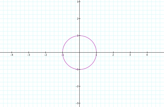
The radius of the circle is one as it should be for the unit circle and since t goes from 0 to 2pi, the whole circle is on the graph. This result makes even more sense when thinking about how the values of a for the equations are both 1. The equation x = cos(t) can be written as x = 1cos(t) and y = sin(t) can be written as y = 1sin(t). Realizing the connection between the value of a and the graph of the equations, I wanted to see what would happen to the graph if I varied the value of a for the equations.
Instead of varying both values of a for the two equations at once, I decided to adjust the value of a for x = cos(t) first. By doing this I am able to see how this particular value of a adjusts the graph of the equations. Below is an illustration of the graph when the value of a varies between -10 and 10 for the equation x = a cos(t).
From this illustration we can see that as the value of the parameter a varies between -10 and 10 for the equation x = a cos(t), the ellipse's width (length across horizontally) also varies. As the parameter a gets farther away from the value of 0, the wider the ellipse becomes. The same holds true for negative values far away from 0. The height (vertical length) remains the same throughout the illustration.
Now I wanted to keep the equation x = cos(t) the same, and vary the parameter a for the equation y = sin(t). By doing this I am able to see how this particular parameter of a adjusts the graph of the equations. Below is an illustration of the graph when the value of a varies between -10 and 10 for the equation y = a sin(t).
From this illustration we can see that as the value of the parameter a varies between -10 and 10 for the equation y = a sin(t), the ellipse's height varies. As the absolute value of the parameter a gets larger, so does the height of the ellipse. The width in this case remains the same throughout the illustration.
Other ways that might be interesting to change the equations to explore other graphs would be to vary the parameter a for the equations x = cos (a*t) and y = sin (a*t). This would be another great way to get students interacting with the mathematics. You could also change the equations by squaring both equations or adding and/or subtracting to the existing equations. To get students more involved with explorations such as this, have them suggest different ways they might alter the equations to explore other graphs. Having them create and be a part of the assignment will help them to feel a part of their learning experience.